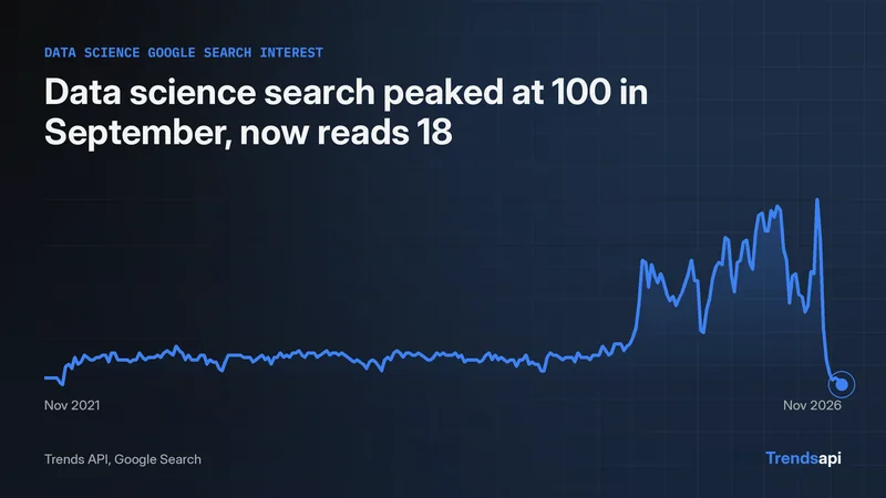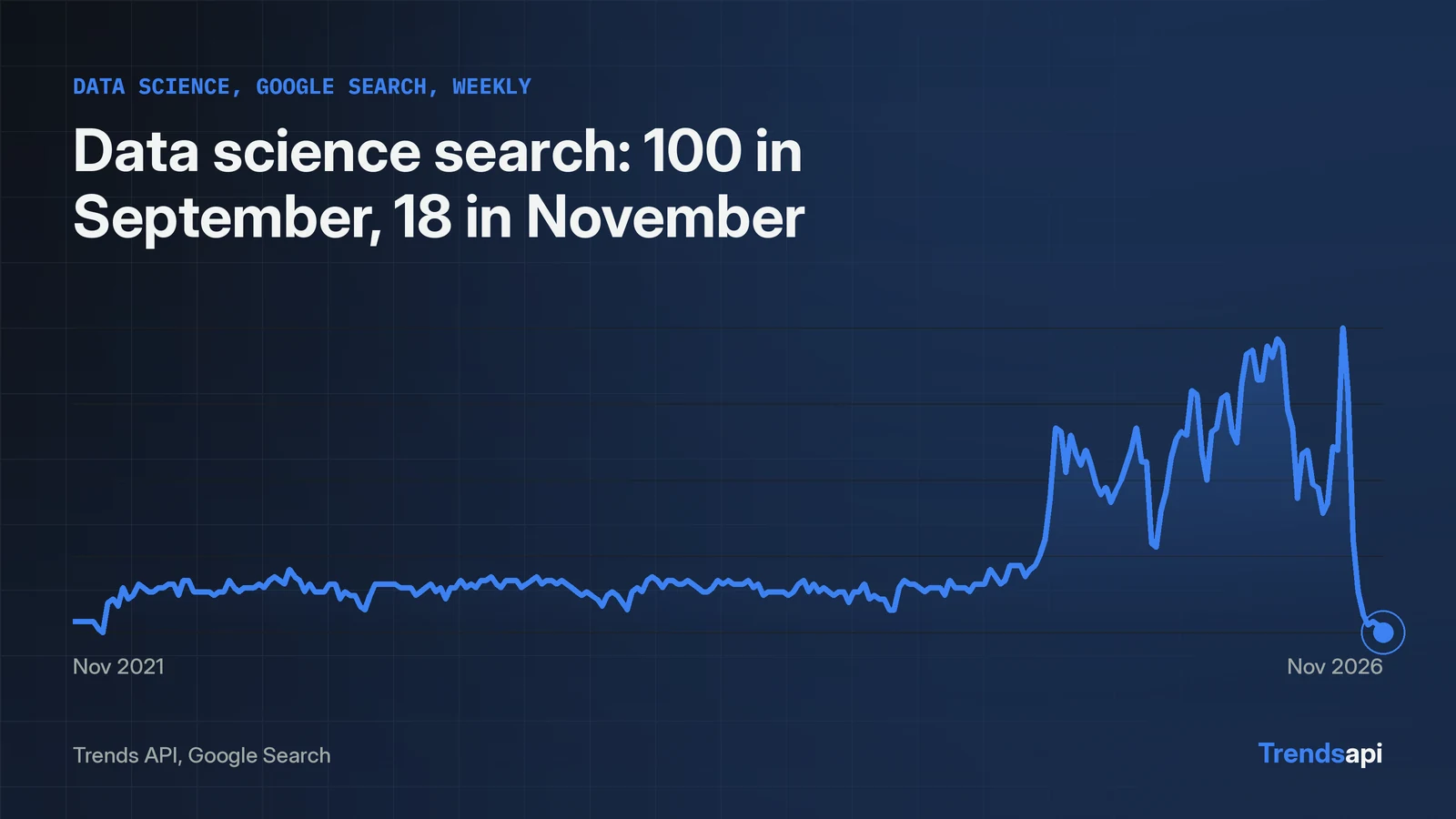
R has no official client for this API, and it does not need one. The whole interface is one POST to https://api.trendsmcp.ai/api with a JSON body, and httr2 sends it in four lines. This page builds a short helper around that call, then uses it four ways: a full history for "data science", growth over two windows, a plot of the series, and a comparison with "machine learning". The requests below were verified live against the API on November 16, 2026, and the R code sends the same URL, headers, and JSON body as the verified calls. "Data science" came back with 261 weekly rows, November 20, 2021 through November 14, 2026, topping out at 100 in the week of September 19, 2026 and closing at 18 on November 14. Request pools by plan are on the pricing page.
Setup: two packages and a key
Install the two packages once, then keep the key out of the script. Getting a key takes an email address and an 8-digit code. No card is asked for.
install.packages(c("httr2", "jsonlite"))
library(httr2)
library(jsonlite)

key <- Sys.getenv("TRENDS_API_KEY")
One helper carries every call
One function serves every mode in this tutorial. It sends the JSON body, unwraps the two-layer reply, and returns a data frame. Nothing else here posts directly.
trends_call <- function(body) {
  resp <- request("https://api.trendsmcp.ai/api") |>
    req_headers(Authorization = paste("Bearer", key)) |>
    req_body_json(body) |>
    req_perform()
  resp_check_status(resp)

  envelope <- resp_body_json(resp)
  fromJSON(envelope$body)
}
The helper earns its keep in two places. The Authorization header takes the key with a Bearer prefix; the bare key on its own also passes, which a live probe confirmed with HTTP 200 on November 16, 2026. And the reply needs two parses: the rows arrive inside an outer object carrying statusCode 200, with the rows themselves stored as a JSON string under body. resp_body_json opens the outer object, fromJSON opens the inner string. Skip the second parse and the code holds a string, not a frame. The resp_check_status line stops the script on an HTTP error instead of parsing an error as data. Leave the key out and the API answers 401, missing_api_key. Send a wrong one and it answers 403, invalid_api_key. Both responses were probed live on November 16, 2026.
A full history in one call
The call below fetches the full history for "data science": 261 weekly rows running November 20, 2021 through November 14, 2026, with the top reading of 100 on September 19. get_time_series is the mode that fetches one keyword on one source, and the body below is the exact body the API received in the live verification run.
series <- trends_call(list(
  mode = "get_time_series",
  keyword = "data science",
  source = "Google Search"
))

series$date <- as.Date(substr(series$date, 1, 10))
nrow(series)  # 261
tail(series, 1)
The frame holds 261 rows, a week apiece from 2021-11-20 through 2026-11-14. Five columns come back on every row: date, value, volume, keyword, and source. Volume rides along on every row: 519,596 on the first, 445,368 on the last. The biggest week is 2026-09-19: index 100, volume 2,474,265. Yearly means tell the longer story: about 30 across 2022, 2023, and 2024, then 44.1 in 2025 and 66.0 in 2026. September's peak lasted one week: 67 on September 12, 100 on September 19, 82 on September 26, then a fall to 18 by November 14 interrupted once, by a rise to 21 on October 31.
Saving the series for later
The CSV preserves the same 261 rows without spending another request. One line writes the frame to disk, and the file can be read back in a later session.
write.csv(series, "data-science-weekly.csv", row.names = FALSE)
The file holds the same 261 rows: date, value, volume, keyword, and source. Re-reading it with read.csv and converting the date column back with as.Date restores the frame. The habit matters because each fresh pull draws on the monthly pool, and a saved CSV costs nothing the second time. The same helper can refill it whenever the data goes stale; the date column shows at a glance how old the file is.
Growth over two windows, then a plot
Growth says the same thing two ways: down 68.42% over three months (57 on August 15 to 18 on November 14) and down 69.49% over twelve months (59 on November 15, 2025 to 18). get_growth measures the latest point against earlier ones, and one call covers both windows.
growth <- trends_call(list(
  mode = "get_growth",
  keyword = "data science",
  source = "Google Search",
  percent_growth = list("3M", "12M")
))
growth
Both windows agree, which is the check that matters: this is a genuine cooling from a September peak, not a weekly wobble. A base R plot shows the shape without another package.
plot(series$date, series$value, type = "l",
     xlab = "Week", ylab = "Index (0-100)",
     main = "Data science, Google Search")
The line holds near 30 for three years, steps up through 2025, spikes to 100 in a single week in September 2026, then drops hard. That shape is why the growth numbers read the way they do, and why a single current value never tells the story on its own.
Comparing two keywords with the same helper
The helper takes any keyword, so a second call puts "data science" next to "machine learning" without new code. Both series have 261 weekly points on Google Search, and both peaked at 100 in 2026, but in different months: machine learning peaked in the week of May 16, 2026, four months before data science peaked on September 19. Both have cooled since. Machine learning read 13 on November 14, down 77.19% in three months from 57 on August 15, and down 66.67% in twelve months from 39 on November 15, 2025. Data science read 18 on the same date. The two series move together closely over five years, with a correlation of 0.95 across 261 weeks, but their peaks fall in different months, which is the useful part: a comparison shows when two related terms move together and when they do not.
ml <- trends_call(list(
  mode = "get_time_series",
  keyword = "machine learning",
  source = "Google Search"
))

ml$date <- as.Date(substr(ml$date, 1, 10))
plot(ml$date, ml$value, type = "l",
     xlab = "Week", ylab = "Index (0-100)",
     main = "Machine learning, Google Search")
What each call costs
The usage call states the rule as of November 16, 2026: a call costs one request for each data type it asks for, a board costs one request per ten rows, and a data type that stays silent costs nothing. That usage call runs over MCP, not REST: over REST the same call answers invalid_mode, and the reference lists it as free over MCP. Check current pricing on the pricing page. The Google Trends API tutorial runs the same calls in Python, and the Search Trends API page lists the five REST tools with their cost in requests.