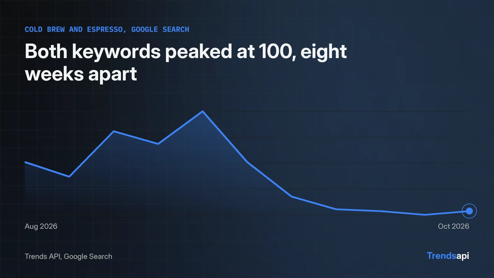
Each keyword's 0 to 100 series is reported on its own scale, so a raw 51 next to a 27 says nothing about absolute search size. The reference defines value as interest on a 0 to 100 index. Both series top out at exactly 100.0 on different dates, which fits each scale being set by that keyword's own peak, though the reference states no formula. Cold brew peaked at 100 on 2026-02-21. Espresso peaked at 100 on 2026-04-18, 56 days later. The fix is to rescale both series over one shared window before comparing shape: subtract the window minimum, divide by the window range. This tutorial pulls both series from the Trends API, lines them up on the 11 shared weeks from 2026-08-22 to 2026-10-31, rescales each to 0 to 1, and checks the volume field where it exists. The code runs in Python with the requests library. One POST to https://api.trendsmcp.ai/api carries every call. All figures are a 2026-11-11 snapshot.
The raw index hides the scale behind each keyword
A 51 for espresso and a 27 for cold brew on 2026-10-31 describe position inside each keyword's own history, not size. The reference defines value as interest on a 0 to 100 index, and gives no formula for the denominator. Both series top out at exactly 100.0, cold brew on 2026-02-21 and espresso on 2026-04-18, which is consistent with each scale being set by that keyword's own peak. That reading is inference, not a documented rule. Cold brew ran 261 weekly points from 2021-11-06 to 2026-10-31, from a low of 15 to its 100 peak. Espresso ran 261 points from 2021-11-13 to 2026-11-07, from a low of 28 to its 100 peak. Two series, two peaks, two different scales. Any chart that plots the raw values side by side compares positions on two different scales, not demand.
One small client pulls both series
One helper posts the JSON body and returns the list of points. The envelope returns body as text, so the code parses it a second time to reach the list. That second parse is easy to miss. The reference states REST always answers HTTP 200 with an envelope carrying statusCode and body, so the code reads statusCode from the envelope and raises on anything but 200 before parsing the body. The call asks for mode get_time_series, source Google Search, and one keyword at a time. The key lives in TRENDSAPI_API_KEY, the variable name the Node.js guide uses.
import json
import os
import requests

API_URL = "https://api.trendsmcp.ai/api"
KEY = os.environ["TRENDSAPI_API_KEY"]

def series(keyword):
    resp = requests.post(API_URL, headers={
        "Authorization": f"Bearer {KEY}",
        "Content-Type": "application/json",
    }, json={"mode": "get_time_series", "keyword": keyword,
             "source": "Google Search"}, timeout=30)
    resp.raise_for_status()
    envelope = resp.json()
    status = envelope.get("statusCode", 200)
    if status != 200:
        raise RuntimeError(f"Trends API {status}: {envelope.get('body')}")
    return json.loads(envelope["body"])

cold_brew = series("cold brew")
espresso = series("espresso")
print(len(cold_brew), cold_brew[0]["date"], cold_brew[-1]["date"])
print(len(espresso), espresso[0]["date"], espresso[-1]["date"])
The run returned 261 points for each keyword. Cold brew covers 2021-11-06 to 2026-10-31. Espresso covers 2021-11-13 to 2026-11-07. Live dates carry a time suffix, so the code below keeps the first 10 characters. A missing week drops out of the shared set, so the last 11 shared weeks reach further back instead of breaking the comparison. Backfill search interest data first when a series comes back short. The Google Trends API tutorial in Python shows the same client pattern with a second keyword and growth windows.
Eleven shared weeks make 0 to 1 comparable
The two series end on different weeks, so the shared window is the 11 weeks both cover: 2026-08-22 to 2026-10-31. These dates are the snapshot as of 2026-11-11. Rerunning the code later shifts the last-11 window. Rescaling uses one formula per keyword: subtract the window minimum, divide by the window range. Cold brew spans 25 to 82 in the window. Espresso spans 51 to 81. Each point lands between 0 and 1, and 1 now marks the window high for that keyword instead of a five-year peak.
def rescale(points, dates):
    by_date = {p["date"][:10]: p["value"] for p in points}
    vals = [by_date[d] for d in dates]
    lo, hi = min(vals), max(vals)
    if hi == lo:
        return [(d, v, 0.0) for d, v in zip(dates, vals)]
    return [(d, v, round((v - lo) / (hi - lo), 3)) for d, v in zip(dates, vals)]

shared = sorted(set(p["date"][:10] for p in cold_brew)
                & set(p["date"][:10] for p in espresso))[-11:]
cold_scaled = rescale(cold_brew, shared)
esp_scaled = rescale(espresso, shared)
for row in cold_scaled:
    print(row)
for row in esp_scaled:
    print(row)
| Week | Cold brew raw | Cold brew 0 to 1 | Espresso raw | Espresso 0 to 1 |
|---|---|---|---|---|
| 2026-08-22 | 54 | 0.509 | 67 | 0.533 |
| 2026-08-29 | 46 | 0.368 | 65 | 0.467 |
| 2026-09-05 | 71 | 0.807 | 81 | 1.000 |
| 2026-09-12 | 64 | 0.684 | 75 | 0.800 |
| 2026-09-19 | 82 | 1.000 | 78 | 0.900 |
| 2026-09-26 | 54 | 0.509 | 76 | 0.833 |
| 2026-10-03 | 35 | 0.175 | 65 | 0.467 |
| 2026-10-10 | 28 | 0.053 | 55 | 0.133 |
| 2026-10-17 | 27 | 0.035 | 54 | 0.100 |
| 2026-10-24 | 25 | 0.000 | 55 | 0.133 |
| 2026-10-31 | 27 | 0.035 | 51 | 0.000 |
The rescaled table reads as shape. Espresso crests at 1.000 on 2026-09-05. Cold brew crests at 1.000 on 2026-09-19. Both slide through October. Cold brew bottoms at 0.000 on 2026-10-24. Espresso bottoms at 0.000 on 2026-10-31. Week-to-week directions agree in 8 of 10 moves and diverge in the last two weeks: from 2026-10-17 to 2026-10-24 cold brew falls while espresso rises, and from 2026-10-24 to 2026-10-31 cold brew rises while espresso falls. Rescaling preserves direction, since it is monotonic per series, so the table shows levels relative to each window, not new direction. On the same weeks, the pairs run 71 vs 81 on 2026-09-05 and 82 vs 78 on 2026-09-19.
Position, not size, is what the level check adds
Rescaling to 0 to 1 erases level. Cold brew ends the shared window at 27 after touching 82. Espresso ends it at 51 after touching 81. Those endpoints describe position, not counts. Pair the rescaled shape with the raw window mean and a percent of that mean. Cold brew averaged 46.6 across the 11 weeks, with a population standard deviation of 19.01. Espresso averaged 65.6, with a population standard deviation of 10.28. On the final week of the shared window, cold brew read 27, or 57.9% of its window mean, a z-score of -1.03. Espresso read 51, or 77.7% of its window mean, a z-score of -1.42. Espresso's actual last point, 2026-11-07 at 52, sits outside the shared window and is excluded from these figures. Espresso ends the window further below its window mean, in standard deviation units, than cold brew does. The mean and the z-score describe position only. They do not turn the index into search counts, and a high raw value can still look like strong demand.
import statistics

def level(points, dates):
    by_date = {p["date"][:10]: p["value"] for p in points}
    vals = [by_date[d] for d in dates]
    mean = statistics.mean(vals)
    sd = statistics.pstdev(vals)
    last = vals[-1]
    if sd == 0:
        return {"mean": round(mean, 1), "sd": 0.0,
                "last_pct_of_mean": round(100 * last / mean, 1),
                "last_z": 0.0}
    return {"mean": round(mean, 1), "sd": round(sd, 2),
            "last_pct_of_mean": round(100 * last / mean, 1),
            "last_z": round((last - mean) / sd, 2)}

print(level(cold_brew, shared))
print(level(espresso, shared))
The code uses the population standard deviation, statistics.pstdev, so the printed 19.01 and 10.28 reproduce exactly. The sample version, statistics.stdev, gives different numbers.
Volume decides size, and it is often absent
Only the volume field carries absolute size, and it is not always there. Cold brew and espresso carry no volume field on any of their 261 points. A separate check on "air fryer" found volume on all 261 points, with the last reading at 3,527,156 on 2026-10-31 and the peak-week volume at 7,504,587 on 2026-05-09. All three checks ran on 2026-11-11. The rule is short: test for the field on the points in hand before using it, and when it is absent, say so and stay with shape. The API reference lists volume as number or null on each series point, which matches what the live calls returned: present for some keywords, missing for others.