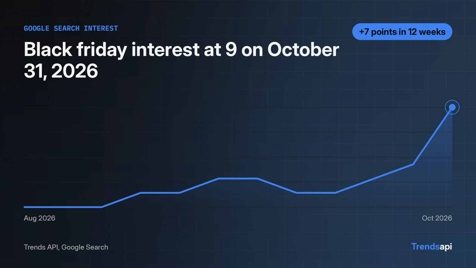
A chart of one Trends API series takes a single API call and a short matplotlib script. The call is a POST to https://api.trendsmcp.ai/api with mode get_time_series, keyword black friday and source Google Search. The response envelope carries the rows as a JSON string inside body, so the code parses twice. The live run returned 261 weekly points from 2021-11-06 to 2026-10-31. The peak reads 100 on 2021-11-27. The latest point reads 9.0 on 2026-10-31. The script below fetches the series, plots dates against values, marks the peak and the latest point, and saves the figure as a PNG.
One POST returns the whole series
get_time_series takes a keyword and exactly one source, and returns about five years of weekly points as a 0 to 100 index. No other parameters are needed for this chart: weekly is the default resolution, and no country is passed. The chart needs one call, and the request limits for each plan sit on the pricing page. The key travels in the Authorization header as Bearer <key>, and the script below reads it from the environment instead of pasting it into the code.
Weekly points are the default, and this piece keeps them. The resolution parameter also takes daily, which returns one point per day for roughly the last three months. That suits a close look at a recent move. The weekly series suits the longer view instead: five years of shape in 261 numbers, with each November spike visible as a single tall point. This chart needs the long view, so weekly stays.
Fetch, parse, plot in one script
import json
import os

import matplotlib
matplotlib.use("Agg")
import matplotlib.pyplot as plt
import requests

KEY = os.environ["TMCP_API_KEY"]
KEYWORD = "black friday"
SOURCE = "Google Search"

resp = requests.post(
    "https://api.trendsmcp.ai/api",
    headers={"Authorization": f"Bearer {KEY}", "Content-Type": "application/json"},
    json={"mode": "get_time_series", "keyword": KEYWORD, "source": SOURCE},
    timeout=60,
)
resp.raise_for_status()
envelope = resp.json()
assert envelope["statusCode"] == 200, envelope
rows = json.loads(envelope["body"])  # the body is a JSON string to parse again
print(f"rows: {len(rows)}")

dates = [r["date"][:10] for r in rows]
values = [r["value"] for r in rows]
peak_idx = values.index(max(values))
print(f"peak: {values[peak_idx]} on {dates[peak_idx]}")
print(f"latest: {values[-1]} on {dates[-1]}")

fig, ax = plt.subplots(figsize=(10, 5))
ax.plot(dates, values, linewidth=1.2)
ax.annotate(
    f"Peak {values[peak_idx]:.0f} on {dates[peak_idx]}",
    xy=(dates[peak_idx], values[peak_idx]),
    xytext=(10, 12),
    textcoords="offset points",
    arrowprops={"arrowstyle": "->"},
)
ax.annotate(
    f"Latest {values[-1]:.1f} on {dates[-1]}",
    xy=(dates[-1], values[-1]),
    xytext=(-8, 12),
    textcoords="offset points",
    ha="right",
    arrowprops={"arrowstyle": "->"},
)
ax.set_title("Google Search interest: black friday")
ax.set_ylabel("Interest (0 to 100)")
ax.set_ylim(0, 110)
plt.xticks(rotation=30)
plt.tight_layout()
fig.savefig("black-friday-chart.png", dpi=150)
print("saved black-friday-chart.png")
The body is a JSON string to parse again
Every answer from the REST endpoint arrives as HTTP 200, and the result sits inside an envelope shaped {"statusCode": 200, "body": "<JSON string>"}. The body field is a JSON string, so json.loads runs a second time to turn it into rows. The assert on statusCode catches query failures, which arrive inside the envelope rather than as HTTP errors.
The live run printed three lines:
rows: 261
peak: 100.0 on 2021-11-27
latest: 9.0 on 2026-10-31
Each row carries date, value, keyword and source. The date strings arrive with a time component attached, so the script slices the first 10 characters to keep the calendar date. The 261 rows cover 2021-11-06 to 2026-10-31, which matches about five years of weekly history for one keyword on one source.
Plot dates against values with one matplotlib call
matplotlib.use("Agg") runs before the pyplot import, and it picks a backend that writes files without a screen. The script runs on a server with no display and still saves the PNG. ax.plot draws the line at width 1.2, thin enough that the yearly November spikes stay sharp instead of blurring into blocks.
The y axis runs 0 to 110, not 0 to 100, so the 100 peak keeps headroom and the annotation arrow has room above it. The x labels rotate 30 degrees so 261 weekly dates do not pile onto each other. Two annotations carry the reading: the peak, 100 on 2021-11-27, and the latest point, 9.0 on 2026-10-31. fig.savefig writes black-friday-chart.png at 150 dpi, and the same file name works as the saved figure for a report or a dashboard.
The annotation offsets are small on purpose. The peak label sits 10 points right and 12 points above its point, with an arrow back to the line. The latest label sits 12 points above the final point and aligns right, so the text stays inside the figure edge instead of running past it. Both labels print the number with one decimal or none, matching the values the API returned: 100 as a whole number, 9.0 with its decimal.
One difference between the page and the script: the hero image at the top of this page shows the last 12 weeks only, while the script plots the full 261-point series. The hero is a close look at the recent ramp. The saved PNG is the whole five years.
What the chart shows about black friday
The line spends most of the year near the floor and spikes each November. The November peak for each year in the series:
| Year | November peak | Date |
|---|---|---|
| 2021 | 100 | 2021-11-27 |
| 2022 | 83 | 2022-11-26 |
| 2023 | 91 | 2023-11-25 |
| 2024 | 89 | 2024-11-30 |
| 2025 | 89 | 2025-11-29 |
The 100 peak in 2021 is the highest point in the whole series. Every later November peak reads lower against it, between 83 and 91. The shape repeats: a flat baseline, then a steep climb into the last week of November.
The last 12 weeks, from the week of August 15 to the week of October 31 2026, read 2, 2, 2, 3, 3, 4, 4, 3, 3, 4, 5, 9. The latest point, 9 on 2026-10-31, is the highest of those 12 weeks. The series was still climbing into the final week of October.
The climb from 2 to 9 looks small next to the November peaks of 83 to 100, and that gap is the point of the 0 to 100 scale. October interest reads as a single digit while November reads near the top, so the chart shows the seasonal shape at a glance: a flat baseline for most of the year, then a steep wall into the last week of November. The 2026 November peak is not in the data yet, because the series ends on 2026-10-31.
Swap the keyword and the labels follow
The script takes one keyword and produces one chart. The peak and latest annotations read their values from the data, so a different keyword needs no other change: the labels move to the new peak and the new latest point on their own, and the y axis still leaves room above 100. That is the whole reuse story. One constant changes, and the figure rebuilds itself around the new series.
The first-calls tutorial covers the same endpoint across more modes: growth windows, a two-keyword comparison, the live boards and context, using matcha as its example. The notebook tutorial runs the same call inside a notebook for readers who plot there. This piece stays on one job: fetch one series, chart it, mark the two points that matter.
FAQ
Why is 2021 the only November to reach 100?
The index scales each series to its own highest point, so 100 marks the series maximum, which fell on 2021-11-27. Later Novembers read lower against that peak: 83 in 2022, 91 in 2023, 89 in 2024 and 89 in 2025.
What does a value of 9 mean?
On a 0 to 100 index, 9 means search interest at 9 percent of the series maximum, the 100 recorded on 2021-11-27. The number is relative to the keyword's own history, not to other keywords, so it describes the shape of this series and nothing else.
Does the script need a display to draw the chart?
No. matplotlib.use("Agg") picks a backend that writes files without a screen, so the script runs on a server and still saves the PNG.